Math
Plotting
- Download
 member dnewman's 3dplot.scad and place it in the same directory as your OpenSCAD file that will use it.
- Create a new OpenSCAD document. Save it as 2dgraphing.scad. Paste this code, which is derived from
user Brad Pitcher, into the empty document:
pi = 3.1415926536; e = 2.718281828; /************************* * Cartesian equations *************************/ /* Sine wave */ module sineWave(){ linear_extrude(height=5) 2dgraph([-50, 50], 3, steps=50); } module parabola (){ linear_extrude(height=5) 2dgraph([-50, 50], 3, steps=40); } /* Ellipsoid - use a cartesion equation for a half ellipse, then rotate extrude it */ module ellipsoid(){ rotate_extrude(convexity=10, $fn=100) rotate([0, 0, -90]) 2dgraph([-50, 50], 3, steps=100); } /************************* * Polar equations *************************/ /* Rose curve */ module rose(){ scale([20, 20, 20]) linear_extrude(height=0.15) 2dgraph([0, 720], 0.1, steps=160, polar=true); } /* Archimedes spiral */ module archimedesSpiral(){ scale([0.02, 0.02, 0.02]) linear_extrude(height=150) 2dgraph([0, 360*3], 50, steps=100, polar=true); } /* Golden spiral */ module goldenSpiral(){ linear_extrude(height=50) 2dgraph([0, 7*180], 1, steps=300, polar=true); } /************************** * Parametric equations *************************/ /* 9-pointed star */ module ninePointedStar(s,h){ scale(s) linear_extrude(height=h) 2dgraph([10, 1450], 0.1, steps=9, parametric=true); } /*************************/ // function to convert degrees to radians function d2r(theta) = theta*360/(2*pi); // These functions are here to help get the slope of each segment, and use that to find points for a correctly oriented polygon function diffx(x1, y1, x2, y2, th) = cos(atan((y2-y1)/(x2-x1)) + 90)*(th/2); function diffy(x1, y1, x2, y2, th) = sin(atan((y2-y1)/(x2-x1)) + 90)*(th/2); function point1(x1, y1, x2, y2, th) = [x1-diffx(x1, y1, x2, y2, th), y1-diffy(x1, y1, x2, y2, th)]; function point2(x1, y1, x2, y2, th) = [x2-diffx(x1, y1, x2, y2, th), y2-diffy(x1, y1, x2, y2, th)]; function point3(x1, y1, x2, y2, th) = [x2+diffx(x1, y1, x2, y2, th), y2+diffy(x1, y1, x2, y2, th)]; function point4(x1, y1, x2, y2, th) = [x1+diffx(x1, y1, x2, y2, th), y1+diffy(x1, y1, x2, y2, th)]; function polarX(theta) = cos(theta)*r(theta); function polarY(theta) = sin(theta)*r(theta); module nextPolygon(x1, y1, x2, y2, x3, y3, th) { if((x2 > x1 && x2-diffx(x2, y2, x3, y3, th) < x2-diffx(x1, y1, x2, y2, th) || (x2 <= x1 && x2-diffx(x2, y2, x3, y3, th) > x2-diffx(x1, y1, x2, y2, th)))) { polygon( points = [ point1(x1, y1, x2, y2, th), point2(x1, y1, x2, y2, th), // This point connects this segment to the next point4(x2, y2, x3, y3, th), point3(x1, y1, x2, y2, th), point4(x1, y1, x2, y2, th) ], paths = [[0,1,2,3,4]] ); } else if((x2 > x1 && x2-diffx(x2, y2, x3, y3, th) > x2-diffx(x1, y1, x2, y2, th) || (x2 <= x1 && x2-diffx(x2, y2, x3, y3, th) < x2-diffx(x1, y1, x2, y2, th)))) { polygon( points = [ point1(x1, y1, x2, y2, th), point2(x1, y1, x2, y2, th), // This point connects this segment to the next point1(x2, y2, x3, y3, th), point3(x1, y1, x2, y2, th), point4(x1, y1, x2, y2, th) ], paths = [[0,1,2,3,4]] ); } else { polygon( points = [ point1(x1, y1, x2, y2, th), point2(x1, y1, x2, y2, th), point3(x1, y1, x2, y2, th), point4(x1, y1, x2, y2, th) ], paths = [[0,1,2,3]] ); } } module 2dgraph(bounds=[-10,10], th=2, steps=10, polar=false, parametric=false) { step = (bounds[1]-bounds[0])/steps; union() { for(i = [bounds[0]:step:bounds[1]-step]) { if(polar) { nextPolygon(polarX(i), polarY(i), polarX(i+step), polarY(i+step), polarX(i+2*step), polarY(i+2*step), th); } else if(parametric) { nextPolygon(x(i), y(i), x(i+step), y(i+step), x(i+2*step), y(i+2*step), th); } else { nextPolygon(i, f(i), i+step, f(i+step), i+2*step, f(i+2*step), th); } } } } - Open another OpenSCAD document.
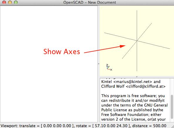
- To display the axes in the model view press Command+2 (MAC) or CTRL+2 (Windows and Linux).
- Save the new document as openscadMath.scad in the same place as you saved the other two documents.
- The first line of the new file should be :
use <2dgraph.scad>
use <3dplot.scad>
- This is how you would create a sine wave:
Press F5 to render
function _f(x) = 20*sin((1/4)*x);
function f(x) = _f(d2r(x));
sineWave();
- Here are some other shapes:
Shape Code Parabola function f(x) = pow(x, 2)/20; parabola();
ellipsoid function f(x) = sqrt((2500-pow(x, 2))/3); ellipsoid();
rose function r(theta) = cos(4*theta); rose();
Archimedes Spiral function r(theta) = theta/2*pi; archimedesSpiral();
Golden Spiral function r(theta) = pow(e, 0.0053468*theta); goldenSpiral();
Nine Pointed Star function x(t) = cos(t); function y(t) = sin(t); ninePointedStar([10,10,10],0.25);
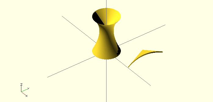
- For the 3d graphing there are four example graphs to play with:
Select one or two, uncomment them and render the 3D graph (F5)Graph Code Square ripples in a pond function z(x,y) = 2*cos(rad2deg(abs(x)+abs(y))); 3dplot([-4*pi,4*pi],[-4*pi,4*pi],[50,50],-2.5);
A wash board function z(x,y) = cos(rad2deg(abs(x)+abs(y))); 3dplot([-4*pi,4*pi],[-4*pi-20,4*pi-20],[50,50],-1.1);
Uniform bumps and dips function z(x,y) = 5*cos(rad2deg(x)) * sin(rad2deg(y)); 3dplot([-2*pi,2*pi],[-2*pi,2*pi],[50,50],-6);
sombrero function function z(x,y) = 15*cos(180*sqrt(x*x+y*y)/pi)/sqrt(2+x*x+y*y); 3dplot([-4*pi,+4*pi],[-4*pi,+4*pi],[50,50],-5);
- OpenSCAD also includes syntax for for loops. Here is an example that takes advantage of the cos() function:
for(i=[0:36]){
    for(j=[0:10]){
        translate([i*10,j*10,0])cylinder(r=5,h=cos(i*10)*50+60);
    }
}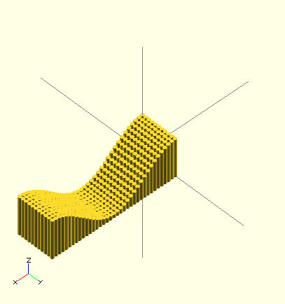
- Here is an example that takes advantage of the sin() function:
for(i=[0:36]){
    for(j=[0:10]){
        translate([i*10,j*10,0])cylinder(r=5,h=sin(i*10)*50+60);
    }
}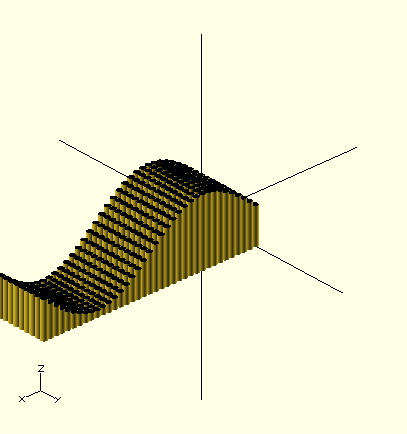
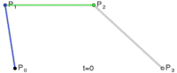
Bézier curves
For a computer to draw a curve, you have to use a mathematical function to describe it.
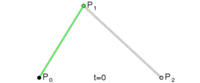
A Bézier curve is a parametric curve.
In vector graphics, Bézier curves are used to model smooth curves that can be scaled indefinitely.
Quadratic and cubic Bézier curves are most common as higher degree curves are more computationally expensive to evaluate. When more complex shapes are needed, low order Bézier curves are patched together. This is commonly referred to as a path in vector graphics. To guarantee smoothness, the control point at which two curves meet must be on the line between the two control points on either side.
Bézier curves were widely publicized in 1962 by the French engineer Pierre Bézier, who used them to design automobile bodies at Renault. The study of these curves was first developed in 1959 by mathematician Paul de Casteljau using de Casteljau's algorithm, a numerically stable method to evaluate Bézier curves, at Citroën, another French automaker.
Images from Wikipedia
The Math Behind the Bézier Curve
A cubic Bézier curve is defined by four points.(x0,y0) is the origin endpoint.
(x3,y3) is the destination endpoint.
The points (x1,y1) and (x2,y2) are control points.
Two equations define the points on the curve. Both are evaluated for an arbitrary number of values of t between 0 and 1. One equation yields values for x, the other yields values for y. As increasing values for t are supplied to the equations, the point defined by x(t),y(t) moves from the origin to the destination. This is how the equations are defined in Adobe's PostScript references.
 x(t) = axt3 + bxt2 + cxt + x0

    x1 = x0 + cx / 3

    x2 = x1 + (cx +bx) / 3

    x3 = x0 + cx +bx + ax
  y(t) = ayt3 + byt2+ cyt + y0

    y1 = y0 + cy / 3

    y2 = y1 + (cy+by) / 3

    y3 = y0 + cy +by+ ay
This method of definition can be reverse-engineered so that it'll give up the coefficient values based on the points described above:
    cx = 3 (x1 - x0)

    bx = 3 (x2 - x1) -cx

    ax = x3 - x0 -cx - bx

    cy = 3 (y1 - y0)

    by = 3 (y2 - y1) -cy

    ay = y3 - y0 -cy - by
Now, simply by knowing coördinates for any four points, you can create the equations for a simple Bézier curve.
From moshplant
For more information about Bézier Curves see processingjs.nihongoresources.com/bezierinfo
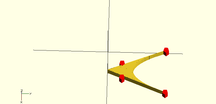
Instructions for Conic or Quadratic Bézier Curves
These curves are named conic because the 3-point Bézier curve is a parabola, which is the intersection of a cone with a plane (i.e. a conic section).- Download the Bézierconic.scad by member donb
- Set p0 and p2 as endpoints ([x,y])
- Set p1 as a control point ([x,y])
- Call the
p0=[10,0];
p1=[0,20];
p2=[10,30];


linear_extrude(height=1) translate([15,0,0]) BezConic(p0,p1,p2,20);

rotate_extrude($fn=100) BezConic(p0,p1,p2,steps=40);
Instructions for Cubic Bézier Curves
- Download the Bézier.scad by member WilliamAAdams
- Create 4 appropriate control points
cPoints=[[0, 20],[5,5],[10,5],[15,20]];
- Choose a focal point. The focalPoint is the point from which all triangle fans will originate.
gFocalPoint=[7.5,0];
- Set the gSteps
gSteps=20;
- Set the gHeight
gHeight=4;
- Call the BezQuadCurve() module
BezQuadCurve( cPoints, gFocalPoint, gSteps, gHeight);
- You can use the PointAlongBez4 function to calculate any point along the Bézier curve defined by your control points, and the u factor (between 0 and 1).
Returns:[0,20]
echo (PointAlongBez4([0, 20],[5,5],[10,5],[15,20], 0));
Returns:[7.5,8.75]echo (PointAlongBez4([0, 20],[5,5],[10,5],[15,20], .5));
Returns:[15,20]echo (PointAlongBez4([0, 20],[5,5],[10,5],[15,20], 1));
Challenge:
Create an interesting math formDesign one object that uses at least one Bézier Curve.
Standards
Mathematics, Science, and Technology
-
STANDARD 1
Analysis, Inquiry, and Design: ENGINEERING DESIGN
Key Idea 1: details
Engineering design is an iterative process involving modeling and optimization (finding the best solution within given constraints); this process is used to develop technological solutions to problems within given constraints. (Note: The design process could apply to activities from simple investigations to long-term projects.)Elementary 1.1 Describe objects, imaginary or real, that might be modeled or made differently and suggest ways in which the objects can be changed, fixed, or improved √ 1.2 Investigate prior solutions and ideas from books, magazines, family, friends, neighbors, and community members √ 1.3 Generate ideas for possible solutions, individually and through group activity; apply age-appropriate mathematics and science skills; evaluate the ideas and determine the best solution; and explain reasons for the choices √ 1.4 Plan and build, under supervision, a model of the solution using familiar materials, processes, and hand tools √ 1.5 Discuss how best to test the solution; perform the test under teacher supervision; record and portray results through numerical and graphic means; discuss orally why things worked or didn't work; and summarize results in writing, suggesting ways to make the solution better √
Intermediate T1.1 Identify needs and opportunities for technical solutions from an investigation of situations of general or social interest. √ T1.1a Identify a scientific or human need that is subject to a technological solution which applies scientific principles √ T1.2 Locate and utilize a range of printed, electronic, and human information resources to obtain ideas. √ T1.2a Use all available information systems for a preliminary search that addresses the need. √ T1.3 Consider constraints and generate several ideas for alternative solutions, using group and individual ideation techniques (group discussion, brainstorming, forced connections, role play); defer judgment until a number of ideas have been generated; evaluate (critique) ideas; and explain why the chosen solution is optimal. √ T1.3a Generate ideas for alternative solutions √ T1.3b Evaluate alternatives based on the constraints of design √ T1.4 Develop plans, including drawings with measurements and details of construction, and construct a model of the solution, exhibiting a degree of craftsmanship. √ T1.4a Design and construct a model of the product or process √ T1.4b Construct a model of the product or process √ T1.5 In a group setting, test their solution against design specifications, present and evaluate results, describe how the solution might have been modified for different or better results, and discuss trade-offs that might have to be made. √ T1.5a Test a design √ T1.5b Evaluate a design √
Commencement 1.1 Initiate and carry out a thorough investigation of an unfamiliar situation and identify needs and opportunities for technological invention or innovation √ 1.2 identify, locate, and use a wide range of information resources including subject experts, library references, magazines, videotapes, films, electronic data bases and online services, and discuss and document through notes and sketches how findings relate to the problem 1.3 generate creative solution ideas, break ideas into the significant functional elements, and explore possible refinements; predict possible outcomes using mathematical and functional modeling techniques; choose the optimal solution to the problem, clearly documenting ideas against design criteria and constraints; and explain how human values, economics, ergonomics, and environmental considerations have influenced the solution √ 1.4 develop work schedules and plans which include optimal use and cost of materials, processes, time, and expertise; construct a model of the solution, incorporating developmental modifications while working to a high degree of quality (craftsmanship) √ 1.5 in a group setting, devise a test of the solution relative to the design criteria and perform the test; record, portray, and logically evaluate performance test results through quanitative, graphic, and verbal means; and use a variety of creative verbal and graphic techniques effectively and persuasively to present conclusions, predict impacts and new problems, and suggest and pursue modifications -
STANDARD 2
INFORMATION SYSTEMS
Key Idea 1: details
Information technology is used to retrieve, process, and communicate information as a tool to enhance learning.Elementary 1.1 Use computer technology,traditional paper-based resources,and interpersonal discussions to learn, do, and share science in the classroom √ 1.2 Select appropriate hardware and software that aids in wordprocessing, creating databases, telecommunications, graphing, data display, and other tasks √ 1.3 Use information technology to link the classroom to world events
Intermediate 1.1 Use a range of equipment and software to integrate several forms of information in order to create good-quality audio, video, graphic, and text-based presentations. 1.2 Use spreadsheets and database software to collect, process, display, and analyze information. Students access needed information from electronic databases and on-line telecommunication services. 1.3 Systematically obtain accurate and relevant information pertaining to a particular topic from a range of sources, including local and national media, libraries, muse- ums, governmental agencies, industries, and individuals. 1.4 Collect data from probes to measure events and phenomena. 1.4a Collect the data, using the appropriate, available tool 1.4b Organize the data 1.4c Use the collected data to communicate a scientific concept √ 1.5 Use simple modeling programs to make predictions.
Physics 1.1 Understand and use the more advanced features of word processing, spreadsheets, and database software. 1.2 Prepare multimedia presentations demonstrating a clear sense of audience and purpose. (Note: Multimedia may include posters, slides, images, presentation software, etc.) √ 1.2a Extend knowledge of physical phenomena through independent investigation, e.g., literature review, electronic resources, library research 1.2b Use appropriate technology to gather experimental data, develop models,and present results √ 1.3 Access, select, collate, and analyze information obtained from a wide range of sources such as research databases, foundations, organizations, national libraries, and electronic communication networks, including the Internet. 1.3a Use knowledge of physics to evaluate articles in the popular press on contemporary scientific topics 1.4 Utilize electronic networks to share information. √ 1.5 Model solutions to a range of problems in mathematics, science, and technology, using computer simulation software. √ 1.5a Use software to model and extend classroom and laboratory experiences,recognizing the differences between the model used for understanding and real-world behavior √ -
STANDARD 5
Technology: Engineering Design
Key Idea 1:details
Engineering design is an iterative process involving modeling and optimization used to develop technological solutions to problems within given constraints.Elementary T1.1 Describe objects, imaginary or real, that might be modeled or made differently and suggest ways in which the objects can be changed, fixed, or improved. √ T1.2 Investigate prior solutions and ideas from books, magazines, family, friends, neighbors, and community members. √ T1.3 Generate ideas for possible solutions, individually and through group activity; apply age-appropriate mathematics and science skills; evaluate the ideas and determine the best solution; and explain reasons for the choices. √ T1.4 Plan and build, under supervision, a model of the solution using familiar materials, processes, and hand tools √ T1.5 Discuss how best to test the solution; perform the test under teacher supervision; record and portray results through numerical and graphic means; discuss orally why things worked or didn't work; and summarize results in writing, suggesting ways to make the solution better. √
Intermediate T1.1 Identify needs and opportunities for technical solutions from an investigation of situations of general or social interest. √ T1.2 Locate and utilize a range of printed, electronic, and human information resources to obtain ideas. √ T1.3 Consider constraints and generate several ideas for alternative solutions, using group and individual ideation techniques (group discussion, brainstorming, forced connections, role play); defer judgment until a number of ideas have been generated; evaluate (critique) ideas; and explain why the chosen solution is optimal. √ T1.4 Develop plans, including drawings with measurements and details of construction, and construct a model of the solution, exhibiting a degree of craftsmanship. √ T1.5 In a group setting, test their solution against design specifications, present and evaluate results, describe how the solution might have been modified for different or better results, and discuss tradeoffs that might have to be made. √
Commencement T1.1 Initiate and carry out a thorough investigation of an unfamiliar situation and identify needs and opportunities for technological invention or innovation. √ T1.2 Identify, locate, and use a wide range of information resources including subject experts, library references, magazines, videotapes, films, electronic data bases and on-line services, and discuss and document through notes and sketches how findings relate to the problem. T1.3 Generate creative solution ideas, break ideas into the significant functional elements, and explore possible refinements; predict possible outcomes using mathematical and functional modeling techniques; choose the optimal solution to the problem, clearly documenting ideas against design criteria and constraints; and explain how human values, economics, ergonomics, and environmental considerations have influenced the solution. √ T1.4 Develop work schedules and plans which include optimal use and cost of materials, processes, time, and expertise; construct a model of the solution, incorporating developmental modifications while working to a high degree of quality (craftsmanship). √ T1.5 In a group setting, devise a test of the solution relative to the design criteria and perform the test; record, portray, and logically evaluate performance test results through quantitative, graphic, and verbal means; and use a variety of creative verbal and graphic techniques effectively and persuasively to present conclusions, predict impacts and new problems, and suggest and pursue modifications. -
STANDARD 5
Technology: Engineering Design
Key Idea 2: details
Technological tools, materials, and other resources should be selected on the basis of safety, cost, availability, appropriateness, and environmental impact; technological processes change energy, information, and material resources into more useful forms.Elementary 2.1 Explore, use, and process a variety of materials and energy sources to design and construct things. √ 2.2 Understand the importance of safety, cost, ease of use, and availability in selecting tools and resources for a specific purpose. 2.3 Develop basic skill in the use of hand tools 2.4 Use simple manufacturing processes (e.g., assembly, multiple stages of production, quality control) to produce a product √ 2.5 Use appropriate graphic and electronic tools and techniques to process information. √
Intermediate 2.1 Choose and use resources for a particular purpose based upon an analysis and understanding of their properties, costs, availability, and environmental impact √ 2.2 Use a variety of hand tools and machines to change materials into new forms through forming, separating, and combining processes, and processes which cause internal change to occur √ 2.3 Combine manufacturing processes with other technological processes to produce, market, and distribute a product 2.4 Process energy into other forms and information into more meaningful information.
Commencement 2.1 Test, use, and describe the attributes of a range of material (including synthetic and composite materials), information, and energy resources √ 2.2 Select appropriate tools, instruments, and equipment and use them correctly to process materials, energy, and information √ 2.3 Explain tradeoffs made in selecting alternative resources in terms of safety, cost, properties, availability, ease of processing, and disposability 2.4 Describe and model methods (including computer-based methods) to control system processes and monitor system outputs √ -
STANDARD 5
Technology: Computer Technology
Key Idea 3: details
Computers, as tools for design, modeling, information processing, communication, and system control, have greatly increased human productivity and knowledge.Elementary 3.1 Identify and describe the function of the major components of a computer system. 3.2 Use the computer as a tool for generating and drawing ideas. √ 3.3 Control computerized devices and systems through programming. √ 3.4 Model and simulate the design of a complex environment by giving direct commands.
Intermediate 3.1 Assemble a computer system including keyboard, central processing unit and disc drives, mouse, modem, printer, and monitor 3.2 Use a computer system to connect to and access needed information from various Internet sites √ 3.3 Use computer hardware and software to draw and dimension prototypical designs √ 3.4 Use a computer as a modeling tool √ 3.5 Use a computer system to monitor and control external events and/or systems √
Commencement 3.1 Understand basic computer architecture and describe the function of computer subsystems and peripheral devices 3.2 Select a computer system that meets personal needs 3.3 Attach a modem to a computer system and telephone line, set up and use communications software, connect to various online networks, including the Internet, and access needed information using email, telnet, gopher, ftp, and web searches 3.4 Use computer-aided drawing and design (CADD) software to model realistic solutions to design problems √ 3.5 Develop an understanding of computer programming and attain some facility in writing computer programs √ -
STANDARD 5
Technology: Impacts of Technology
Key Idea 6: details
Technology can have positive and negative impacts on individuals, society, and the environment and humans have the capability and responsibility to constrain or promote technological development.Elementary 6.1 Describe how technology can have positive and negative effects on the environment and on the way people live and work. √
Intermediate 6.1 Describe how outputs of a technological system can be desired, undesired, expected, or unexpected 6.2 Describe through examples how modern technology reduces manufacturing and construction costs and produces more uniform products
Commencement 6.1 Explain that although technological effects are complex and difficult to predict accurately, humans can control the development and implementation of technology. 6.2 Explain how computers and automation have changed the nature of work 6.3 Explain how national security is dependent upon both military and nonmilitary applications of technology -
STANDARD 5
Technology: Management of Technology
Key Idea 7: details
Project management is essential to ensuring that technological endeavors are profitable and that products and systems are of high quality and built safely, on schedule, and within budget.Elementary 7.1 Participate in small group projects and in structured group tasks requiring planning, financing, production, quality control, and follow-up. √ 7.2 Speculate on and model possible technological solutions that can improve the safety and quality of the school or community environment.
Intermediate 7.1 Manage time and financial resources in a technological project 7.2 Provide examples of products that are well (and poorly) designed and made, describe their positive and negative attributes, and suggest measures that can be implemented to monitor quality during production 7.3 Assume leadership responsibilities within a structured group activity √
Commencement 7.1 Develop and use computer-based scheduling and project tracking tools, such as flow charts and graphs 7.2 Explain how statistical process control helps to assure high quality output 7.3 Discuss the role technology has played in the operation of successful U.S. businesses and under what circumstance they are competitive with other countries 7.4 Explain how technological inventions and innovations stimulate economic competitiveness and how, in order for an innovation to lead to commercial success, it must be translated into products and services with marketplace demand 7.5 Describe new management techniques (e.g., computer-aided engineering, computer-integrated manufacturing, total quality management, just-in-time manufacturing), incorporate some of these in a technological endeavor, and explain how they have reduced the length of design-to-manufacture cycles, resulted in more flexible factories, and improved quality and customer satisfaction 7.6 Help to manage a group engaged in planning, designing, implementation, and evaluation of a project to gain understanding of the management dynamics √ -
STANDARD 6
Interconnectedness: Common Themes SYSTEMS THINKING:
Key Idea 1: details
Through systems thinking, people can recognize the commonalities that exist among all systems and how parts of a system interrelate and combine to perform specific functions.Elementary 1.1 Observe and describe interactions among components of simple systems. √ 1.2 Identify common things that can be considered to be systems (e.g., a plant population, a subway system, human beings).
Intermediate 1.1 Describe the differences between dynamic systems and organizational systems. 1.2 describe the differences and similarities between engineering systems, natural systems, and social systems. 1.3 Describe the differences between open- and closed-loop systems. 1.4 Describe how the output from one part of a system (which can include material, energy, or information) can become the input to other parts.
Commencement 1.1 Explain how positive feedback and negative feedback have opposite effects on system outputs. 1.2 Use an input-process-output-feedback diagram to model and compare the behavior of natural and engineered systems. 1.3 Define boundary conditions when doing systems analysis to determine what influences a system and how it behaves. -
STANDARD 6
Interconnectedness: Common Themes OPTIMIZATION:
Key Idea 6: details
In order to arrive at the best solution that meets criteria within constraints, it is often necessary to make trade-offs.Elementary 6.1 Choose the best alternative of a set of solutions under given constraints. √ 6.2 Explain the criteria used in selecting a solution orally and in writing √
Intermediate 6.1 Determine the criteria and constraints and make trade-offs to determine the best decision. √ 6.2 Use graphs of information for a decision-making problem to determine the optimum solution.
Physics Determine optimal solutions to problems that can be solved using quantitative methods √ -
STANDARD 7
Interdisciplinary Problem Solving STRATEGIES:
Key Idea 2: details
Solving interdisciplinary problems involves a variety of skills and strategies, including effective work habits; gathering and processing information; generating and analyzing ideas; realizing ideas; making connections among the common themes of mathematics, science, and technology; and presenting results.Physics 2.1 Collect,analyze,interpret,and present data,using appropriate tools √ 2.2 When students participate in an extended,culminating mathematics,science,and technology project, then students should: Work effectively—Contributing to the work of a brainstorming group, laboratory partnership, cooperative learning group, or project team; planning procedures; identify and managing responsibilities of team members; and staying on task, whether working alone or as part of a group. √ Gather and process information —Accessing information from printed media, electronic data bases, and community resources and using the information to develop a definition of the problem and to research possible solutions. √ Generate and analyze ideas — Developing ideas for proposed solutions, investigating ideas, collecting data, and showing relationships and patterns in the data. √ Observe common themes—Observing examples of common unifying themes, applying them to the problem, and using them to better understand the dimensions of the problem. √ Realize ideas—Constructing components or models, arriving at a solution, and evaluating the result. √ Present results—Using a variety of media to present the solution and to communicate the results. √
CDOS
- Standard 2: Integrated Learning
details
Students will demonstrate how academic knowledge and skills are applied in the workplace and other settings.
Integrated learning encourages students to use essential academic concepts, facts, and procedures in applications related to life skills and the world of work. This approach allows students to see the usefulness of the concepts that they are being asked to learn and to understand their potential application in the world of work.
Elementary 2.1 Identify academic knowledge and skills that are required in specific occupations 2.2 Demonstrate the difference between the knowledge of a skill and the ability to use the skill 2.3 Solve problems that call for applying academic knowledge and skills. √
Intermediate 2.1 Apply academic knowledge and skills using an interdisciplinary approach to demonstrate the relevance of how these skills are applied in work-related situations in local, state, national, and international communities 2.2 Solve problems that call for applying academic knowledge and skills √ 2.3 Use academic knowledge and skills in an occupational context, and demonstrate the application of these skills by using a variety of communication techniques (e.g., sign language, pictures, videos, reports, and technology).
Commencement 2.1 Demonstrate the integration and application of academic and occupational skills in their school learning, work, and personal lives. √ 2.2 Use academic knowledge and skills in an occupational context, and demonstrate the application of these skills by using a variety of communication techniques (e.g., sign language, pictures, videos, reports, and technology) √ 2.3 Research, interpret, analyze, and evaluate information and experiences as related to academic knowledge and technical skills when completing a career plan. - Standard 3a: Universal Foundation Skills
details
Students will demonstrate mastery of the foundation skills and competencies essential for success in the workplace.
- Basic skills
Basic skills include the ability to read, write, listen, and speak as well as perform arithmetical and mathematical functions.
Elementary 3.1.1 Listen to and read the ideas of others and express themselves both orally and in writing; they use basic mathematical concepts and computations to solve problems. √
Intermediate 3.1.1 Listen to and read the ideas of others and analyze what they hear and read; acquire and use information from a variety of sources; and apply a combination of mathematical operations to solve problems in oral or written form. √
Commencement 3.1.1 Use a combination of techniques to read or listen to complex information and analyze what they hear or read; convey information confidently and coherently in written or oral form; and analyze and solve mathematical problems requiring use of multiple computational skills. √ - Thinking skills
Thinking skills lead to problem solving, experimenting, and focused observation and allow the application of knowledge to new and unfamiliar situations.
Elementary 3.2.1 Use ideas and information to make decisions and solve problems related to accomplishing a task. √
Intermediate 3.2.1 Evaluate facts, solve advanced problems, and make decisions by applying logic and reasoning skills. √
Commencement 3.2.1 Demonstrate the ability to organize and process information and apply skills in new ways. √
- Personal Qualities
Personal qualities generally include competence in self-management and the ability to plan, organize, and take independent action.
Elementary 3.3.1 Demonstrate the personal qualities that lead to responsible behavior. √
Intermediate 3.3.1 Demonstrate the ability to work with others, present facts that support arguments, listen to dissenting points of view, and reach a shared decision. √
Commencement 3.3.1 Demonstrate leadership skills in setting goals, monitoring progress, and improving their performance. √
- Interpersonal Skills
Positive interpersonal qualities lead to teamwork and cooperation in large and small groups in family, social, and work situations.
Elementary 3.4.1 Relate to people of different ages and from diverse backgrounds.
Intermediate 3.4.1 Demonstrate the ability to work with others, present facts that support arguments, listen to dissenting points of view, and reach a shared decision. √
Commencement 3.4.1 Communicate effectively and help others to learn a new skill. √
- Technology
Technology is the process and product of human skill and ingenuity in designing and creating things from available resources to satisfy personal and societal needs and wants.
Elementary 3.5.1 Demonstrate an awareness of the different types of technology available to them and of how technology affects society.
Intermediate 3.5.1 Select and use appropriate technology to complete a task. √
Commencement 3.5.1 Apply their knowledge of technology to identify and solve problems. √
- Managing Information
Information management focuses on the ability to access and use information obtained from other people, community resources, and computer networks.Elementary 3.6.1 Describe the need for data and obtain data to make decisions. √
Intermediate 3.6.1 Select and communicate information in an appropriate format (e.g., oral, written, graphic, pictorial, multimedia). √
Commencement 3.6.1 Use technology to acquire, organize, and communicate information by entering, modifying, retrieving, and storing data. √
- Managing Resources
Using resources includes the application of financial and human factors, and the elements of time and materials to successfully carry out a planned activity.Elementary 3.7.1 Demonstrate an awareness of the knowledge, skills, abilities, and resources needed to complete a task. √
Intermediate 3.7.1 Understand the material, human, and financial resources needed to accomplish tasks and activities. √
Commencement 3.7.1 Allocate resources to complete a task. √
- Systems
Systems skills include the understanding of and ability to work within natural and constructed systems.Elementary 3.8.1 Demonstrate understanding of how a system operates and identify where to obtain information and resources within the system. √
Intermediate 3.8.1 Understand the process of evaluating and modifying systems within an organization. √
Commencement 3.8.1 Demonstrate an understanding of how systems performance relates to the goals, resources, and functions of an organization. √
- Basic skills
Career Development and Occupational Studies
Standards-based education addresses three types of standards
- content—identify what students should know and be able to do
- performance—identify levels of achievement in relation to the content standards, answering the question "How good is good enough?"
- opportunity-to-learn—the availability of resources, programs, and qualified teachers needed to enable the students to meet the identified standards.
Meeting CDOS Standards means:
- Learning experiences have real-life applications.
- Lessons are authentic and project-based.
- Lessons are experiential in nature.
- Lessons are hands-on.
- Lessons connect to careers.
- Students are able to connect present learning to future goals.
- Students explore various career paths without limiting their choices.
- Students engage in career role-playing.
- Students learn and then apply skills they learn in school.
- Students participate in entrepreneurial endeavors in the school environment.
- Students integrate knowledge with experience.
- Students offer comments of how much they are looking forward to their future careers because classroom activities are relevant to the real world.
- The teacher discusses his/her own skills with students.
- Assessment directly measures performance.
-
Standard 2:details
Integrated Learning
Students will demonstrate how academic knowledge and skills are applied in the workplace and other settings.
Integrated learning encourages students to use essential academic concepts, facts, and procedures in applications related to life skills and the world of work. This approach allows students to see the usefulness of the concepts that they are being asked to learn and to understand their potential application in the world of work.
Elementary 2.1 Identify academic knowledge and skills that are required in specific occupations 2.2 Demonstrate the difference between the knowledge of a skill and the ability to use the skill 2.3 Solve problems that call for applying academic knowledge and skills. √
Intermediate 2.1 Apply academic knowledge and skills using an interdisciplinary approach to demonstrate the relevance of how these skills are applied in work-related situations in local, state, national, and international communities 2.2 Solve problems that call for applying academic knowledge and skills √ 2.3 Use academic knowledge and skills in an occupational context, and demonstrate the application of these skills by using a variety of communication techniques (e.g., sign language, pictures, videos, reports, and technology).
Commencement 2.1 Demonstrate the integration and application of academic and occupational skills in their school learning, work, and personal lives. √ 2.2 Use academic knowledge and skills in an occupational context, and demonstrate the application of these skills by using a variety of communication techniques (e.g., sign language, pictures, videos, reports, and technology) √ 2.3 Research, interpret, analyze, and evaluate information and experiences as related to academic knowledge and technical skills when completing a career plan. - Standard 3a: details
Universal Foundation Skills Students will demonstrate mastery of the foundation skills and competencies essential for success in the workplace.
- Basic skills
Basic skills include the ability to read, write, listen, and speak as well as perform arithmetical and mathematical functions.
Elementary 3.1.1 Listen to and read the ideas of others and express themselves both orally and in writing; they use basic mathematical concepts and computations to solve problems. √
Intermediate 3.1.1 Listen to and read the ideas of others and analyze what they hear and read; acquire and use information from a variety of sources; and apply a combination of mathematical operations to solve problems in oral or written form. √
Commencement 3.1.1 Use a combination of techniques to read or listen to complex information and analyze what they hear or read; convey information confidently and coherently in written or oral form; and analyze and solve mathematical problems requiring use of multiple computational skills. √ - Thinking skills
Thinking skills lead to problem solving, experimenting, and focused observation and allow the application of knowledge to new and unfamiliar situations.
Elementary 3.2.1 Use ideas and information to make decisions and solve problems related to accomplishing a task. √
Intermediate 3.2.1 Evaluate facts, solve advanced problems, and make decisions by applying logic and reasoning skills. √
Commencement 3.2.1 Demonstrate the ability to organize and process information and apply skills in new ways. √
- Personal Qualities
Personal qualities generally include competence in self-management and the ability to plan, organize, and take independent action.
Elementary 3.3.1 Demonstrate the personal qualities that lead to responsible behavior. √
Intermediate 3.3.1 Demonstrate the ability to work with others, present facts that support arguments, listen to dissenting points of view, and reach a shared decision. √
Commencement 3.3.1 Demonstrate leadership skills in setting goals, monitoring progress, and improving their performance. √
- Interpersonal Skills
Positive interpersonal qualities lead to teamwork and cooperation in large and small groups in family, social, and work situations.
Elementary 3.4.1 Relate to people of different ages and from diverse backgrounds.
Intermediate 3.4.1 Demonstrate the ability to work with others, present facts that support arguments, listen to dissenting points of view, and reach a shared decision. √
Commencement 3.4.1 Communicate effectively and help others to learn a new skill. √
- Technology
Technology is the process and product of human skill and ingenuity in designing and creating things from available resources to satisfy personal and societal needs and wants.
Elementary 3.5.1 Demonstrate an awareness of the different types of technology available to them and of how technology affects society.
Intermediate 3.5.1 Select and use appropriate technology to complete a task. √
Commencement 3.5.1 Apply their knowledge of technology to identify and solve problems. √
- Managing Information
Information management focuses on the ability to access and use information obtained from other people, community resources, and computer networks.Elementary 3.6.1 Describe the need for data and obtain data to make decisions. √
Intermediate 3.6.1 Select and communicate information in an appropriate format (e.g., oral, written, graphic, pictorial, multimedia). √
Commencement 3.6.1 Use technology to acquire, organize, and communicate information by entering, modifying, retrieving, and storing data. √
- Managing Resources
Using resources includes the application of financial and human factors, and the elements of time and materials to successfully carry out a planned activity.Elementary 3.7.1 Demonstrate an awareness of the knowledge, skills, abilities, and resources needed to complete a task. √
Intermediate 3.7.1 Understand the material, human, and financial resources needed to accomplish tasks and activities. √
Commencement 3.7.1 Allocate resources to complete a task. √
- Systems
Systems skills include the understanding of and ability to work within natural and constructed systems.Elementary 3.8.1 Demonstrate understanding of how a system operates and identify where to obtain information and resources within the system. √
Intermediate 3.8.1 Understand the process of evaluating and modifying systems within an organization. √
Commencement 3.8.1 Demonstrate an understanding of how systems performance relates to the goals, resources, and functions of an organization. √
- Basic skills
- Standard 3b: details
Career Majors Students who choose a career major will acquire the career-specific technical knowledge/skills necessary to progress toward gainful employment, career advancement, and success in postsecondary programs.- Business/Information Systems
Core 3b.1 Basic Business Understanding—demonstrate an understanding of business, marketing, and multinational economic concepts, perform business-related mathematical computations, and analyze/interpret business-related numerical information. 3b.2 Business-Related Technology—select, apply, and troubleshoot hardware and software used in the processing of business transactions. 3b.3 Information Management/Communication—prepare, maintain, interpret/analyze, and transmit/ distribute information in a variety of formats while demonstrating the oral, nonverbal, and written communication skills essential for working in today's international service-/information-/technological-based economy. 3b.4 Business Systems—demonstrate an understanding of the interrelatedness of business, social, and economic systems/subsystems.
Specialized 3b.5 Resource Management—identify, organize, plan, and allocate resources (e.g., financial, materials/facilities, human, time) in demonstrating the ability to manage their lives as learners, contributing family members, globally competitive workers, and self-sufficient individuals.
Experiential 3b.1 Basic Business Understanding—demonstrate an understanding of business, marketing, and multinational economic concepts, perform business-related mathematical computations, and analyze/interpret business-related numerical information. 3b.2 Business-Related Technology—select, apply, and troubleshoot hardware and software used in the processing of business transactions. 3b.3 Information Management/Communication—prepare, maintain, interpret/analyze, and transmit/ distribute information in a variety of formats while demonstrating the oral, nonverbal, and written communication skills essential for working in today's international service-/information-/technological-based economy. 3b.4 Business Systems—demonstrate an understanding of the interrelatedness of business, social, and economic systems/subsystems. 3b.5 Resource Management—identify, organize, plan, and allocate resources (e.g., financial, materials/facilities, human, time) in demonstrating the ability to manage their lives as learners, contributing family members, globally competitive workers, and self-sufficient individuals. 3b.6 Interpersonal Dynamics—exhibit interpersonal skills essential for success in the multinational business world, demonstrate basic leader- ship abilities/skills, and function effectively as members of a work group or team. - Engineering/Technologies
Core, Specialized and Experiential 3b.1 Foundation Development—Develop practical understanding of engineering technology through reading, writing, sample problem solving, and employment experiences. 3b.2 Technology—Demonstrate how all types of engineering/technical organizations, equipment (hardware/software), and well-trained human resources assist and expedite the production/distribution of goods and services 3b.3 Engineering/Industrial Processes—Demonstrate knowledge of planning, product development and utilization, and evaluation that meets the needs of industry.
- Business/Information Systems
Essential Questions
details| Who am I as a citizen? | Students develop self-management skills for researching a topic. Students develop critical thinking skills. Students develop effective interpersonal skills. | |
| How are my school experiences connected to my future success? | Students will acquire skills in decision making, communication, and teamwork. Students will learn various management skills. Students will participate in a simulated work environment. | |
| How are my social skills related to my future success? | Students will predict future situations. Students will work as a team to complete a project. Students will develop problem-solving strategies. Students will interact effectively with team partners. | |
| How do I develop the skills and abilities that I need to be successful in a career? How do I find out what I want to know? | Students will research topics using the internet | |
| Why do the choices I make now matter to my future? | Students will gain an awareness of the importance of personal responsibility and good work habits. Students will gain an awareness of the impact of their actions and choices. | |
| How do I affect the systems within which I live and work? |
| Business/Information Systems (3b) | |
| Basic Business Understanding | |
| Business-Related Technology | |
| Information Management/ Communication | |
| Business Systems | |
| Resource Management | |
| Interpersonal Dynamics | |
| Career Development (1) | |
| Complete development of career plan | |
| Apply decision-making skills in selection of a career option | |
| Analyze skills and abilities in a career option | |
| Integrated Learning (2) | |
| Demonstrate integration and application | |
| Use academic knowledge and skills | |
| Research, interpret, analyze, and evaluate information | |
| Universal Foundation Skills (3a) | |
| Basic Skills | |
| Thinking Skills | |
| Personal Qualities | |
| Interpersonal Skills | |
| Technology | |
| Managing Information | |
| Managing Resources | |
| Systems | |
/*assignment part 2*/
